The following graphs were prepared using data from the California Independent System Operator (CISO) with one hour resolution from 1 January 2011 until 30 November 2020, and five minute resolution thereafter, data from the Electric Reliability Council of Texas (ERCOT) with hourly resolution from 2 July 2018, data from New York Independent System Operator with five minute resolution from 9 December 2015, nationwide data from the Hourly Electric Grid Monitor with one hour resolution since 1 July 2018, and data from EU for Denmark, Germany, and EU as a whole with hourly resolution from 1 January 2015 until 30 September 2020. They show the net energy content (or deficit) that would have been in storage, assuming all supply came from renewable sources, storage charge and discharge are 100% efficient, and batteries can be fully charged and discharged without damage. At first, the analyses assume a system with unlimited but empty storage capacity at the beginning of the study period. Analyses are repeated with bounded storage capacity.
In early sections, quantities in storage were calculated by assuming average renewable capacity is equal to average demand. In later sections, the effect of average renewable supply being larger than average demand is analyzed. The method of calculation used here is explained below.
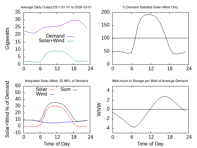
The bottom left graph shows the average daily trend for solar and wind output, as a fraction of average total demand during the period of analysis.
The top right graph shows what fraction of total demand would be satisfied by solar and wind, if they were the only sources and their average output were magnified to equal average demand.
The bottom right graph shows the average daily variation of the amount of energy that would be in storage if solar and wind were the only sources and their average output were magnified to equal average demand. The vertical axis is watt hours in storage per watt of average solar + wind production. This rather rosy average-day picture is the basis for claims that only small amounts of storage are necessary. But look carefully and you'll notice that the average daily deficit is four watt hours per watt, while the average surplus is three watt hours per watt: Storage is being continuously depleted.
Some days are better than average, and some are worse. It is necessary to consider the cumulative effect of good and bad days, especially the cumulative effect of consecutive good and bad days.
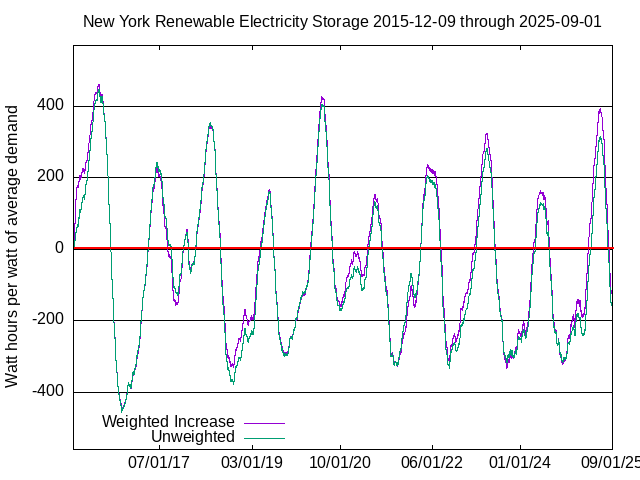
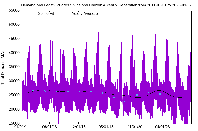
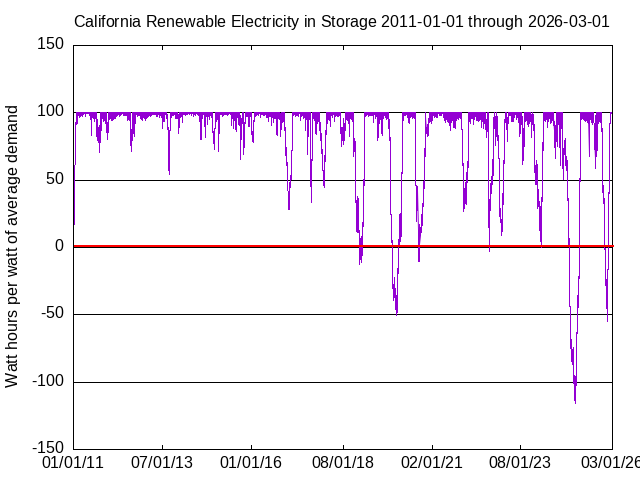
The graph below shows the amount of electrical energy that would have been in storage in California with an all-renewable energy system having average output equal to average demand. The units of the vertical axis are watt hours in storage per watt of average demand, compared to the amount in storage on 1 January 2011.
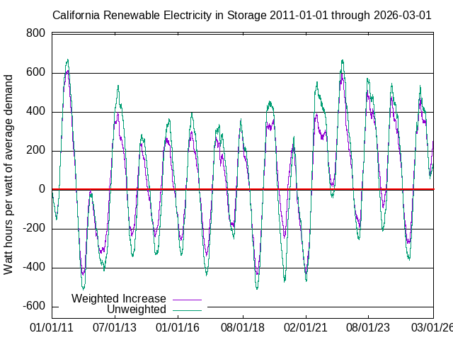
The “Unweighted” (green) line multiplies the outputs of all renewable generators by the same factor so that their total average output is equal to average demand. It is unlikely that biomass, biofuel, and hydro can grow much. Environmentalists want to remove dams, and they complain that fracking for geothermal causes earthquakes.
The “Weighted Increase” (purple) line is computed by magnifying each renewable's output in proportion to the rate of change of that generation method's label capacity, with a different rate for each method in each year.
The maximum surplus calculated using “Weighted Increase” was 626 watt hours per watt on 16 August 2011. The deepest deficit was 453 watt hours per watt on 30 March 2012. To avoid outages and to avoid dumping power when more is available than demand, and storage is already charged to full capacity, a storage system would need to have a capacity of 626 + 453 = 1,079 watt hours per watt of average demand (almost 50 days), and to have been precharged to 453 watt hours per watt of average demand on 1 January 2011 to avoid outages. The effect of precharging would be to shift the graphs upward by 453 watt hours, and the “Weighted Increase” (purple) line would nowhere have been negative.
The yearly average maximum and minimum were 372.6 watt-hours per watt and -198.9 watt-hours per watt, an annual swing of 571.5 watt-hours per watt. The surplus-deficit cycle clearly has a period of a year. Although there would, on average, be daily charge-discharge cycles of about 7 watt hours per watt of average demand, during their ten year lifetimes, batteries would be nearly fully charged and discharged ten times. To break even on operating (not capital) costs, they would need to sell electricity at 57 times the usual rate. This assumes that batteries could hold the surplus for six months until it is needed, and wouldn't be damaged by deep discharge cycles.
Renewable sources provided 39.6% of electrical energy. Without storage and with only renewable sources, when the trend of the amount was negative (δ(t) below is less than zero), i.e., 17.3% of the time, there would have been outages. With unlimited storage capacity, not precharged, when the amount in storage was negative and the trend of the amount was negative, i.e., 6.7% of the time, there would have been outages (see How the Graphs are Computed below). The industry definition of firm power is 99.97% availability, or about two hours and forty minutes of outage per year.
Tbe eleven-year solar cycle is clearly visible.
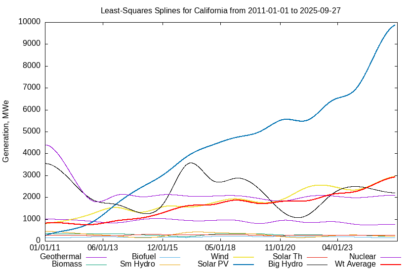
Total label generating capacity amounts, year by year, for each generation method, were obtained from the California Department of Energy.
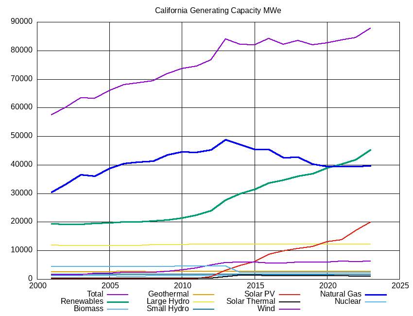
The rate of change of total renewables’ label generating capacity has not changed significantly since 2012, when solar PV began increasing rapidly, and wind and solar thermal stopped increasing.
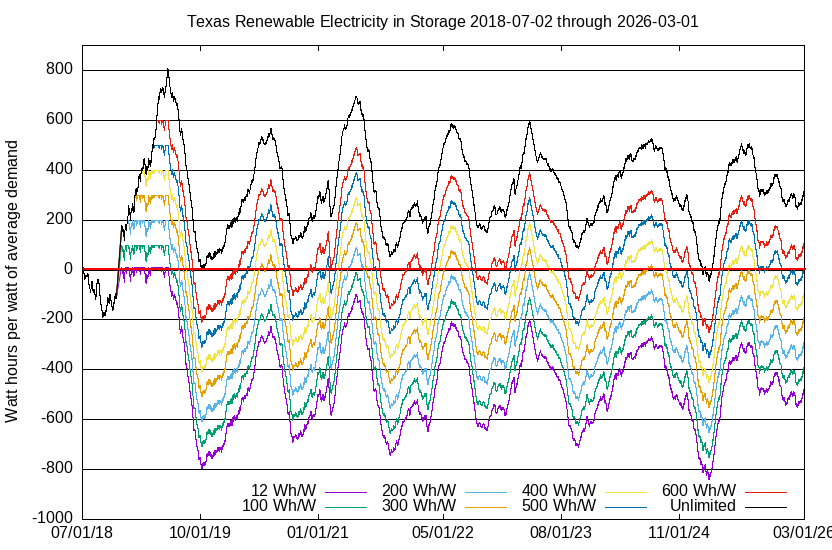
| As of 30 April 2023 | ||
|---|---|---|
| Storage | Outage | Dumped |
| 12 Wh/W | 46.8% | 1.69% |
| 100 Wh/W | 44.4% | 1.69% |
| 200 Wh/W | 41.9% | 1.58% |
| 300 Wh/W | 37.1% | 1.35% |
| 400 Wh/W | 31.6% | 1.12% |
| 500 Wh/W | 26.9% | 0.88% |
| 600 Wh/W | 18.1% | 0.65% |
| Unlimited | 4.4% | 0% |
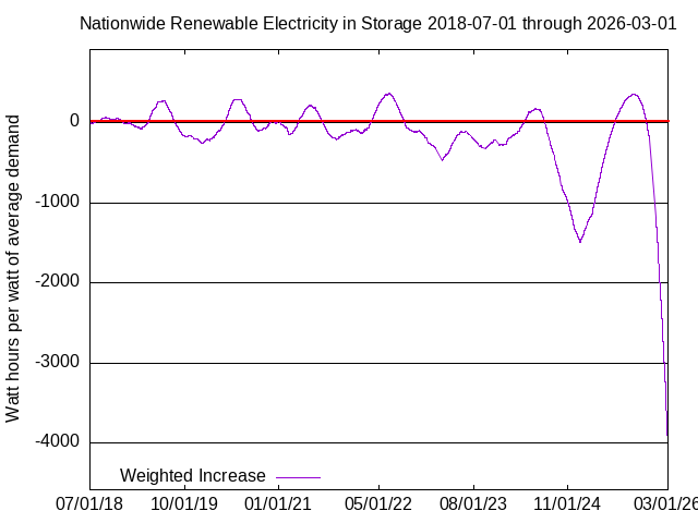
Renewable sources provided 10.33% of nationwide electric energy, or about 3% of total energy. Without storage and with only renewable sources, when the trend of the amount was negative (δ(t)<0), i.e., 56.6% of the time, there would have been outages. With unlimited storage capacity, not precharged, when the amount in storage was negative and the trend of the amount was negative, i.e., 22.7% of the time, there would have been outages. At the current EIA battery price of $0.56/Wh and ten year lifetime, the cost for battery storage to provide firm power would be eighteen times total USA GDP -- every year -- forever.
The May 2020 price for Tesla PowerWall 2 was $0.543 per watt hour (not kilowatt hour) of capacity, including associated electronics but not including installation. Individual installation costs range from $0.142 to $0.214 per watt hour of capacity. Industrial scale systems might get price breaks.
Activists insist that an all-electric United States energy economy would have average demand of about 1,700 GWe. Assume that the California requirement of 1,079 watt hours of storage per watt of average demand is adequate forever (this is optimistic). The total cost for Tesla PowerWall 2 storage units, not including installation, with watt hours' capacity would be quadrillion, or about 58 times total US 2018 GDP (about $20 trillion). Assuming batteries last ten years (the Tesla warranty period), the cost would be 4.98 times total US 2018 GDP per year. The cost for each of America's 128 million households would be about $777,862 per year. If the more pessimistic nationwide analysis is used, the total cost would be 7.9 times total US 2018 GDP per year, and the cost per household would be $1,242,094 per year. Prices that include installation would be 25-40% greater. This very optimistic analysis assumes 100% battery charge and discharge efficiency, and that batteries can hold a 100% charge for six months or more. Lithium ion batteries lose capacity more rapidly at full charge. It is recommended to store them at 50% capacity and moderately low temperatures. If they become completely discharged they are permanently damaged. They're closer to 90% efficient (81% round-trip), so the necessary capacity increase due to efficiency consideration alone would add about 25% more. Taking both installation and the necessary capacity increase into account results in a 75% cost increase to about 13.8 times total GDP every year. Doubling the capacity for optimal long-term storage, and to avoid complete discharge, would increase the cost to about 27.6 times total GDP every year.
Elon Musk would have more money than God.
California average electricity demand is 26 gigawatts. The 1,700 GWe average demand that activists insist an all-electric American energy economy would have is about 3.83 times total current average electricity demand of 444 GWe. Assuming the same ratio for California, total electricity demand in an all-electric California economy would be 99.6 GWe, so the total storage required would be 99.6×109×1,233 = 123 trillion watt hours. The cost for California would be $6.7 trillion per year, or “only” about three times total California GDP every year, or about 5.25 times total California GDP when accounting for installation and 81% round-trip efficiency.
The energy density of lithium ion batteries is 230 watt hours per kilogram. A capacity of 1.9×10¹⁵ watt hours for the entire USA would weigh 8.26 billion tonnes. A lithium ion battery contains the following ingredients (among others):
| Metal's | Metal's Amount in | Metal's | ||||
|---|---|---|---|---|---|---|
| Proportion in | 8.26 billion tonnes | Global | ||||
| Metal | Li-ion Battery | of Li-Ion Batteries | Reserves | Requirement | ||
| (%) | (million tonnes) | (million tonnes) | ÷ Reserve | |||
| Copper | 17.0% | 1,404 | 830 | 1.69 | ||
| Aluminum | 8.5% | 702 | 32,000 | 0.022 | ||
| Nickel | 15.2% | 1,256 | 89.0 | 14.1 | ||
| Cobalt | 2.8% | 231 | 6.9 | 33.5 | ||
| Lithium | 2.2% | 182 | 14.0 | 13.0 | ||
| Graphite | 22.0% | 1,817 | 330.0 | 5.51 |
Other than aluminum, the Earth does not contain enough metals to make the first generation of necessary batteries for the United States alone! Batteries last about ten years, and are not completely recyclable. Even if the first generation could be built, where would the second generation come from?
Presented with these quantities, activists propose other methods, such as pumping water up mountains. In California, where would we get the water and where would we put it? The Oroville Dam at 771 feet or 235 meters is the highest dam in the country. The area of Yosemite Valley is 6 square miles, or about 15 square kilometers. Assuming it's flat (which it isn't), building a 235 meter dam across the entrance could impound 3.525 trillion liters, or 3.525 trillion kilograms, of water. The mouth of the valley is 1,200 meters above sea level, so the top of the full reservoir would be 1,435 meters above sea level. The potential energy, in joules (watt-seconds), of a mass m lifted to a height h in a gravitational field with acceleration g (9.8 meters per second squared at the surface of the Earth) is mgh. Assuming a power plant at sea level, not at the base of the dam, the water in such a reservoir would have potential energy of about 3.525×1012×1,435×9.8/3,600 = 13.8 trillion watt hours. The Betz limit for the efficiency of a turbine is 57%. California would need at least 104 trillion / (0.57×11.5 trillion) = 13.2 of these reservoirs. If the power plant were at the mouth of the valley instead of at sea level, about 81 would be required. The nation as a whole would need almost 1,500. All of this assumes 100% efficiency (after accounting for the Betz limit) and optimal conditions, so in reality much more would be required.
Opportunities for reservoirs the size of Yosemite Valley are limited. The Snowy 2 project in Australia is to connect two reservoirs with capacity of 254099 million liters, separated by an elevation of 680 meters. Water is to be pumped between the reservoirs in 27 kilometers of tunnels (Yosemite Valley is 250 kilometers from San Francisco Bay). Capacity as calculated above would be 470 GWe-hours. The advertised efficiencies are 67-76% depending on output of 1,000-2,000 MWe, or 315-357 GWe-hours. Craig Brooking and Michael Bowden provided a detailed technical report.
The United States would need 9,600 systems equivalent to Snowy 2. There are currently 1,450 conventional hydroelectric power plants, and 40 pumped storage plants, in the United States. The current budget for Snowy 2 is $AU 4.8 billion = $US 3.26 billion, but many expect the project to exceed $AU 20 billion = $US 13.6 billion. The project is scheduled to be completed in 2028, but many believe it will not be completed. The total cost for 9,600 such projects in the United States would be $130 trillion — if we could find places for them and water to use them.
Total rainfall in a particular river's watershed is cyclical. In 2022, Lake Mead was almost empty. Texas has a more difficult problem than California, with water in the East but no mountains, and mountains 1,000 miles to the West but no water. A statistical analysis of data from the Shuttle Radar Topography Mission showed that Kansas is indeed as flat as a pancake.
The next proposal is towing weights up mountains or old mine shafts. How many are required? The storage requirement is 1,722 Wh/W × 1,700,000,000,000 W × 3600 seconds/hour = 16.9 quintillion watt seconds, or joules. Assuming 100% efficiency, a ten tonne weight, and a one kilometer lift, the result is “only” 102 million such devices. Where would these be put? How much would they cost, per year, taking into account capital, amortization, operations, maintenance, safety, replacement, decommissioning, environmental effects, and disposal or recycling?
The next proposal is hydrogen. The end-to-end electrolyzer-to-fuel-cell efficiency of hydrogen is 22%. The end-to-end electrolyzer-to-gas-turbine efficiency is about 7%. Average renewables' capacity would need to be fourteen times larger than average demand. Renewables' capacity factors are about 25%, so label capacity would need to be 55 times larger than average demand. This moves some of the materials problem noted above from batteries to generators. It is possible to store hydrogen overnight, or for a few days, but the real storage problem is yearly, as the graphs show. Hydrogen leaks through every metal, embrittling it by damaging the crystal and micrograin structures. Methane is easier to store. After the massive methane leak under Kathleen Brown's ranch (Jerry “Moonbeam” Brown's sister), why is anybody seriously proposing to store hydrogen underground?
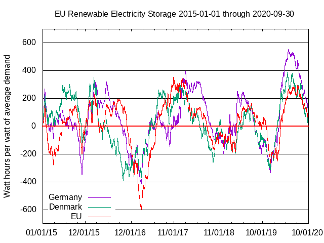
During the interval for which data were available, renewables provided 11.4% of electricity for EU as a whole, 46% for Denmark, and 28.3% for Germany. If solar and wind had been the only generators, for EU as a whole, the largest surplus in storage of unlimited capacity would have been 355 watt hours per watt of average demand, and the deepest deficit would have been 598 watt hours per watt.
To provide firm power without dumping energy when batteries are fully charged, 355 + 598 = 953 watt hours of storage capacity per watt of average demand would have been needed. Without storage and without other generation sources, there would have been outages 55.5% of the time, i.e., whenever the slopes of the lines in this graph are negative. Although the patterns for EU as a whole, and for Denmark and Germany alone, are different, the storage situation is almost identical for Germany: 969 watt hours of storage would be required, and there would have been outages 55.2% of the time without storage if the only generators were renewable sources. Denmark fared somewhat better, requiring only 783 watt hours storage, and would have had outages 54.9% of the time without storage and if the only generators were renewable sources.
The amount of energy in storage at time t since the beginning of the analysis, in watt hours per watt of average demand, is then obtained by accumulating the instantaneous power surplus (or deficit) δ(t) in each measurement interval, multiplied by the interval length (energy = power × time), i.e., computing the integral:
where δ(t) has units of watts of surplus (or deficit) per watt of average demand, N is the number of measurement instants, Δtn (the duration of a measurement interval) has units of hours, and S(t) has units of watt hours per watt of average demand. S(t) is plotted in the graphs.
Rectangular quadrature is justified by the fine resolution of measurements
— Δ
To use historical data to compute what δ(t) would have been if
all sources were renewable sources, it is necessary to increase measured
renewables' average production to match average demand. Let
be current average renewables' production, and
be the additional average renewables' production needed to match average total
demand
where
is a weighted average of renewables' production, and M is a
magnification factor. Then
, or
To compute the relationship of S(t) to average total demand,
that is, how much storage capacity is needed per watt of average demand, we need
where G is a general growth factor that allows to increase the weighted average of renewables' production above average demand,
and
As remarked above, gi(t) were computed as the rate of change of each renewable's generating method, separately in each year for California, and once using a projection for nationwide generation. Therefore, for California, the proportions by which different methods are increased are different each year, and the accumulated surplus (or deficit) of energy in storage is computed as if the generation capacities had been magnified, during that year, to be sufficient to meet average demand. The relationships of rates of increase have not significantly changed in California since about 2012, when solar photovoltaic capacity began increasing rapidly, and construction of new wind capacity stopped. If all gi(t) were equal and constant, this method would assume that all renewable sources can be magnified by the same amount so as to increase their total average output to total average demand (the green line in the graphs). This is not going to happen. For example, environmentalists want to remove dams, not build more of them. In the initial analysis we assumed G = 1. Later, we examine the effect of larger G.
Because neither average demand nor average renewables' production are constant, the “instantaneous” average demand and production were computed using least-squares fits to C2-continuous cubic splines, with constraints on the slopes (mi) at the ends of the interval given by least-squares fits to straight lines, . The slope constraints are necessary because the interval of analysis does not necessarily begin or end at the end of a year. Without it, the “instantaneous” average near the beginning or end of the interval would be anomalously small or large compared to a similar instant in the middle of the interval. (A “cubic spline” is a piecewise curve composed of cubic polynomials. The “C2-continuous” term means that its value, slope, and curvature are continuous everywhere.)
The “Wt Average” line here is for the weighted average .
An example of this method to compute the “instantaneous” average is illustrated for total demand. The end point yearly averages might be anomalously large and small compared to other years when data are available for only a fraction of those years. The “Yearly Average” mark is placed at January 1 of each year.
These analyses are simplistically optimistic. There are several factors not considered that would increase the storage requirement by amounts not quantified here:
Observe that in mid 2020, total energy that would be in storage as a result of all renewables being increased equally, and renewables having produced more than demand, was about 400 watt hours per average watt of capacity. When the amount in storage is negative, for example between November 2020 and June 2021, any time that demand exceeds supply, i.e., δ(t) < 0, there would be outages.
If an all-renewable generating system had been in place in California on 1 January 2011, with a storage system having capacity less than about 1,180 watt hours per watt of average demand, and had not been precharged to 706 watt hours per watt of average demand, there would have been prolonged outages.
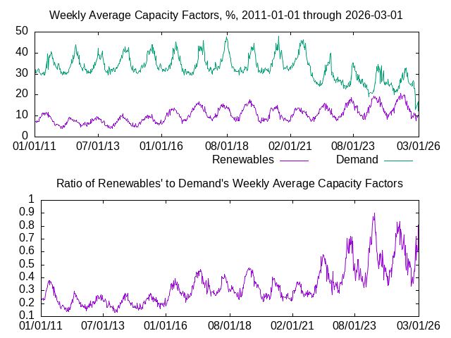
The yearly periodic asynchronous relationship of renewables' output compared to demand is evident in the second graph above.
Phases of yearly variation were computed by fitting each phenomenon to β1 sin ( ω t ) + β2 cos ( ω t ), where ω = 2 π / 8765.81 (the number of hours per year), and t is time in hours since the beginning of the period of analysis (1 January 2011). The phase of each phenomenon with respect to the beginning of the period of analysis is then tan-1 ( β2 / β1 ), and the difference in phases is 46 days, i.e., demand begins to increase about 46 days after output from renewable sources begins to decline.
With the limited amount of data available (fourteen years), by fitting to β1 sin ( ω t ) + β2 cos ( ω t ) + β3 sin ( λ t ) + β4 cos ( λ t ), where ω is as above and λ is to be found, a longer term variation with a period of 8.24 years was found. The phase differences of this variation, tan-1 ( β4 / β3 ), compared to demand, range from -28 days (wind) to +172 days (solar) to +515 days (hydro). The average phase difference between demand and renewables is 45 days. Each time that more data are used, the solved-for period ( λ / 2 π ) increases. Long-term variation frequencies are probably related to the Sun's eleven year activity cycle. There might be even longer term variations that are related to solar activity cycles of about 70 and 1,500 years, but these cannot be measured by using only fourteen years of generation data.
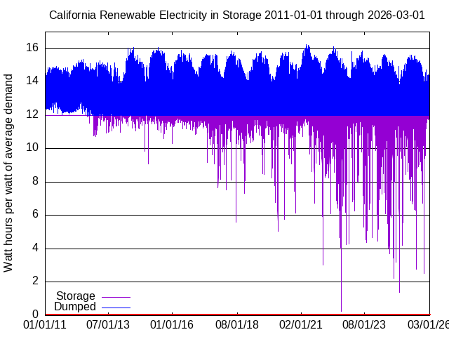
California data were analyzed again with average renewables' generating capacity increased to G = 1.25 times average demand, with the same relative output magnifications gi(t), and a 100 Wh/W storage capacity. The “flat line” bounding the maximum storage amount means that excess generation would be dumped. Solar thermal and wind output can be adjusted somewhat but solar PV output cannot be adjusted if the panels have fixed mountings. Articulated mountings would be very expensive. 776,000 gigawatt hours of output — 44% of total demand — would have been dumped. There would have been outages 19% of the time, i.e., when the slope of the line in this graph is negative.
If average renewables' generating capacity were to have been increased to G = 3 times average demand, and 12 hours' storage were provided, as is claimed to be sufficient by many activists, there would have been outages 3.4% of the time, i.e., when the slope of the line in this graph is negative. 6,300,000 gigawatt hours of output — 355% of total demand — would have been dumped.
The cost for only twelve hours' storage, for an all-electric 1.7 TWe American energy economy, would be $11.1 trillion, or about $1.1 trillion per year, or 5.5% of total GDP. The cost for each of America's 128 million households would be about $8,654 per year for batteries alone.
Renewables provided 33.4% of California electricity between 1 January 2011 and 1 January 2023. Electricity satisfies about one third of total California energy demand. To provide all California energy from renewable electricity sources whose average generating capacity is three times average demand would require a capacity increase of 3 × 3 / 0.334 = 2695% above the capacity to satisfy all current California electricity demand. Increasing hydro at all, or increasing biogas, biomass and geothermal by 2695%, is unlikely. Activists demanded, and California and Oregon acquiesced, that three dams on the Klamath river be removed to restore salmon habitat. Unusually heavy rainfall wiped out that salmon habitat because the dams' flood-control function no longer existed.
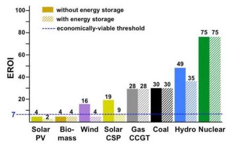
Dumping output reduces the energy return on energy invested (EROI). EROI at least seven is required for economic viability. With storage, and even without dumping, solar PV and wind are not viable without subsidies. Subsidies do not eliminate costs — they just hide them in your tax bill where politicians hope you won't notice them — so they do not actually make solar and wind viable. California appears to have stopped building solar thermal generators — the Ivanpah Solar Electric Generating System is being removed, and the EIA does not predict any increase in US solar thermal capacity.
Daniel Wei�bach, G. Ruprecht, A. Huke, K, Czerski, S. Gottlieb, and A. Hussein, Energy intensities, EROIs (energy returned on invested), energy payback times of electricity generating plants, Energy 52, 1 (April 2013) pp 210-221
Preprint at https://festkoerper-kernphysik.de/Weissbach_EROI_preprint.pdf
D. Wei�bach, F. Herrmann, G. Ruprecht, A. Huke, K, Czerski, S. Gottlieb, and A. Hussein, Energy Intensities, EROI (energy return on invested), for energy sources, EPJ Web of Conferences 189, 00016 (2028) https://www.epj-conferences.org/articles/epjconf/pdf/2018/24/epjconf_eps-sif2018_00016.pdf
If 355% of total renewables' output were dumped, the EROI from solar PV would be reduced to 0.56, i.e., less energy would be produced than invested in the devices. Where would that extra required energy come from? The EROI from wind would be reduced to 1.13.
Every time I read a proposal to put solar panels into orbit, I ask the author what EROI would be. None have replied.
This discussion assumes that the period analyzed includes the deepest deficit that will ever occur — which is, of course, false. When Mount Tambora on the island of Sumbawa in Indonesia erupts again and produces another “year without a summer” such as in 1816 — and it or another one as large definitely will, the only question is when — there will be no times for several years when δ(t) > 0. The trend of storage content will always and everywhere be downward. The deepest deficit will be far deeper than any shown here. No physically feasible or economically viable amount of storage could suffice. Renewable generation capacity and storage capacity could not be increased sufficiently rapidly. There would be energy available for only a small fraction of demand. Politicians' homes, and (maybe) hospitals, would have first priority. Civilization would collapse.
Typos? Mistakes? Quibble with the analysis? Want the software and data I used?
van dot snyder at sbcglobal dot net. 2024 November 26.